How to utilize NiaPy for solving KNN parameter optimization problem?
In the following, I’m going to present to you, an example on how to utilize NiaPy micro-framework 1 for solving the parameter optimization problem of K-nearest neighbors classifier 2 against very common Breast Cancer Wisconsin (Diagnostic) Data Set 3.
Before we dive in, I suppose you are familiar with the basic understanding of machine learning and the usage of the conventional classifiers such as K-nearest neighbors classifier.
If you are only interested in the implementation part you can jump to an Implementation section or view the complete source code on GitHub.
What is NiaPy?
Straight out of the official NiaPy’s documentation site, NiaPy1 is:
“Python micro-framework for building nature-inspired algorithms. Nature-inspired algorithms are a very popular tool for solving optimization problems. Since the beginning of their era, numerous variants of nature-inspired algorithms were developed. To prove their versatility, those were tested in various domains on various applications, especially when they are hybridized, modified or adapted. However, implementation of nature-inspired algorithms is sometimes a difficult, complex and tedious task. In order to break this wall, NiaPy is intended for simple and quick use, without spending a time for implementing algorithms from scratch.”
What do we need?
Before we get started, make sure you have already installed:
- Python (3.6+): download here
- NiaPy: install with pip command
pip install NiaPy - Keras (with Tensorflow):
pip install tensorflow keras - Numpy:
pip install numpy - Scikit-learn:
pip install scikit-learn - pygal (optional charting library):
pip install pygal
Let’s define a problem!
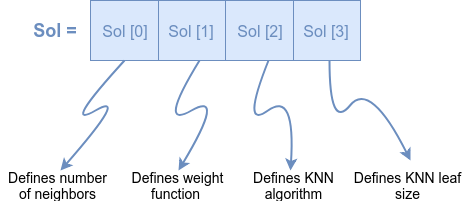
Our problem consists of 4 variables for which we must find the most optimal solution in order to improve classification accuracy of K-nearest neighbors classifier. Those variables are:
- number of neighbors,
- weight function,
- KNN algorithm and
- KNN leaf size.
For finding the most optimal value for each of the mentioned variables, we will utilize the NiaPy micro-framework with one of its embedded nature-inspired algorithm - the Hybrid Bat Algorithm 4.
But before we jump into the implementation of the problem, we need to define the problem in a more formal manner. Probably the most straightforward way to do so is to present the problem as the one-dimensional matrix, with the same number of items as is the number of problem variables. In our case, we will present our problem as shown in Figure 1.
We need to solve just one more thing. The algorithm will pass to our fitness function such one-dimensional matrix (solution) filled with real values between 0 and 1. In order to make those real values useful in the building stage of our classifier, we must map those values into, for us, a bit more meaningful values. For mapping the values, we define following formulas:
Map number of neighbors: $\mathbf{y_1} = \lfloor x[i] * 10 + 5 \rfloor ; y_1 \in [5, 15]$
Map weights: $\mathbf{y_2} = \begin{cases} 1 & \text{if }x[i] > 0.5, \\\ 0 & \text {otherwise } \end{cases}$
Map KNN algorithms: $\mathbf{y_3} = \begin{cases} \lfloor x[i] * 3 + 1 \rfloor ; y_3 \in [1, 3] & \text{if }x[i] < 1, \\\ 3 & \text {otherwise } \end{cases}$
Map KNN leaf size: $\mathbf{y_4} = \lfloor x[i] * 40 + 10 \rfloor ; y_4 \in [10, 50]$
As presented in formulas, the number of neighbors is mapped from real value to the integer number in the range [5, 15]. The weights variable is mapped into 0 or 1, algorithms are mapped to integer range [1, 3] and leaf size is converted to integer range [10, 50].
Implementation time
In this section, we will implement:
- formulas for mapping values defined in the previous section,
- our custom benchmark using those mappers,
- and finally tie together all those pieces into working example.
Firstly, let’s create a new file and name it run.py. Now we implement the mapping formulas in form of function definitions - for each formula, one function definition (see code snippet below).
As you can see, I also added to arrays KNN_WEIGHT_FUNCTIONS and KNN_ALGORITHMS. The purpose of those arrays is to use the mapped values of swap_weights and swap_algorithm as indexes, which will come in handy while building classifiers based on the solution, which has parameters for weight function and algorithm consumes string values instead of numbers.
KNN_WEIGHT_FUNCTIONS = [
    'uniform',
    'distance'
]

KNN_ALGORITHMS = [
    'ball_tree',
    'kd_tree',
    'brute'
]

# map from real number [0, 1] to integer ranging [5, 15]
def swap_n_neighbors(val):
    return int(val * 10 + 5)

# map from real number [0, 1] to integer ranging [0, 1]
def swap_weights(val):
    if val > 0.5:
        return 1
    return 0

# map from real number [0, 1] to integer ranging [1, 3]
def swap_algorithm(val):
    if val == 1:
        return 3
    return int(val * 3 + 1)

# map from real number [0, 1] to integer ranging [10, 50]
def swap_leaf_size(val):
    return int(val * 40 + 10)
Next, we will implement our custom benchmark. Let’s create a new class called KNNBreastCancerBenchmark. In initialization function of the class, we should define the Lower and Upper bound, which are
defining the range of real-values passed (in our case between 0 and 1) in the solution. Afterward, we have to define a function which returns a function with parameters dimension of the problem (D) and
solution array (solution). This function should also return the fitness value of the received solution, so we also need to calculate it. The calculation of fitness values will be implemented as an inverse of test accuracy, which will be implemented in a separate class KNNBreastCancerClassifier inside evaluate function. We would also like to save each solution and the belonging fitness value, so we will append each of them to a scores array. The following is the code snippet of implementation.
class KNNBreastCancerBenchmark(object):
    def __init__(self):
        self.Lower = 0
        self.Upper = 1

    def function(self):
        # our definition of fitness function
        def evaluate(D, solution):
            n_neighbors = swap_n_neighbors(solution[0])
            weights = KNN_WEIGHT_FUNCTIONS[swap_weights(solution[1])-1]
            algorithm = KNN_ALGORITHMS[swap_algorithm(solution[2])-1]
            leaf_size = swap_leaf_size(solution[3])

            fitness = 1 - KNNBreastCancerClassifier().evaluate(n_neighbors, weights, algorithm, leaf_size)

            scores.append([fitness, n_neighbors, weights, algorithm, leaf_size])

            return fitness
        return evaluate
Now, let’s tie those things together. Firstly we will create a new class called KNNBreastCancerClassifier. Inside the initialization function, we set the set the seed value, optionally received through the parameter of init function. Also, inside initialization, we prepare two dictionaries for storing the results of ten-fold cross-validation, while also loading the Breast Cancer Wisconsin (Diagnostic) Data Set. Next, the features and the predicted class is separated from the loaded dataset and stored into variables X and Y. Further, the initial dataset is divided into search and validation splits in ratio 80:20. The smaller subset is furthermore divided into two, train and test subsets in the same ratio as previously. The mentioned, the smaller subset is used to search for most optimal parameters of our classifier, while the larger dataset is used for validation, using ten-fold cross-validation.
Next, we implement the evaluate function, which consumes four parameters: number of neighbors (n_neighbors), weight function (weights), the algorithm used (algorithm) and a leaf size(leaf_size). based on those parameters, the classifier is constructed utilizing the scikit-learn library. After construction of the model, we train mentioned model and run score function against the model to obtain the test accuracy, which we return to the caller of the function.
Finally, we implement a run_10_fold function, which optionally receives the solution as the parameter. In case the solution is passed to the function, the classifier is built using the passed solution parameter, while in other cases the classifier with the default parameters is constructed. In both cases, we then create ten-fold cross-validation split using StratifiedKFold from scikit-learn and we perform mentioned validation using cross_validate function, also from scikit-learn. The only difference between those two cases, beside the mentioned, is that in the first case we perform validation on the whole initial dataset, while in the other case, we perform the validation on the bigger subset as previously described. At last, the results of performed validation are stored into the variables initialized in the init method of the class.
class KNNBreastCancerClassifier(object):
    def __init__(self, seed=1234):
        self.seed = seed
        self.ten_fold_scores = {}
        self.default_ten_fold_scores = {}
        np.random.seed(self.seed)

        dataset = datasets.load_breast_cancer()
        self.X = dataset.data
        self.y = dataset.target

        self.X_search, self.X_validate, self.y_search, self.y_validate = train_test_split(self.X, self.y, test_size=0.8, random_state=self.seed)
        self.X_search_train, self.X_search_test, self.y_search_train, self.y_search_test = train_test_split(self.X_search, self.y_search, test_size=0.8, random_state=self.seed)


    def evaluate(self, n_neighbors, weights, algorithm, leaf_size):
        model = KNeighborsClassifier(n_neighbors=n_neighbors, weights=weights, algorithm=algorithm, leaf_size=leaf_size)
        model.fit(self.X_search_train, self.y_search_train)
        return model.score(self.X_search_test, self.y_search_test)

    def run_10_fold(self, solution=None):
        if solution is None:
            estimator = KNeighborsClassifier()
            kfold = StratifiedKFold(n_splits=10, shuffle=True, random_state=self.seed)
            self.default_ten_fold_scores = cross_validate(estimator, self.X, self.y, cv=kfold, scoring=['accuracy'])
        else:
            estimator = KNeighborsClassifier(n_neighbors=solution[1], weights=solution[2], algorithm=solution[3], leaf_size=solution[4])
            kfold = StratifiedKFold(n_splits=10, shuffle=True, random_state=self.seed)
            self.ten_fold_scores = cross_validate(estimator, self.X_validate, self.y_validate, cv=kfold, scoring=['accuracy'])
Additionally, at the beginning of the file, we need to import the dependencies.
import numpy as np
from sklearn import datasets
from sklearn.neighbors import KNeighborsClassifier
from sklearn.model_selection import train_test_split
from sklearn.model_selection import StratifiedKFold
from sklearn.model_selection import cross_validate
from NiaPy.algorithms.modified import HybridBatAlgorithm
Run and compare the results
Finally, let’s run the example. In the snippet below, is code, which utilizes the NiaPy’s Hybrid Bat Algorithm 4 against our previously written, custom benchmark class. Additionally is the code for printing out the best-found solution for parameters of our classifier.
scores = []
algorithm = HybridBatAlgorithm(4, 40, 100, 0.9, 0.1, 0.001, 0.9, 0.0, 2.0, KNNBreastCancerBenchmark())
best = algorithm.run()

print('Optimal KNN parameters are:')
best_solution = []

for score in scores:
    if score[0] == best:
        best_solution = score

print(best_solution)
Now, we will test our classifier based on the best solution, against classifier with the default parameter settings using well known ten-fold cross-validation method.
model = KNNBreastCancerClassifier()
model.run_10_fold(solution=best_solution)
model.run_10_fold()

print('best model mean test accuracy: ' + str(np.mean(model.ten_fold_scores['test_accuracy'])))
print('default model mean test accuracy: ' + str(np.mean(model.default_ten_fold_scores['test_accuracy'])))
Int the following table are presented the results of test accuracy across each fold, as well as the mean accuracy.
| Default model | Best model | |
|---|---|---|
| Fold-1 | 96.55% | 95.65% |
| Fold-2 | 81.03% | 97.83% |
| Fold-3 | 96.49% | 95.65% |
| Fold-4 | 92.98% | 93.48% |
| Fold-5 | 92.98% | 95.65% |
| Fold-6 | 92.98% | 86.96% |
| Fold-7 | 94.73% | 95.65% |
| Fold-8 | 96.43% | 88.89% |
| Fold-9 | 92.86% | 88.86% |
| Fold-10 | 91.07% | 93.18% |
| Mean | 92.81% | 93.18% |
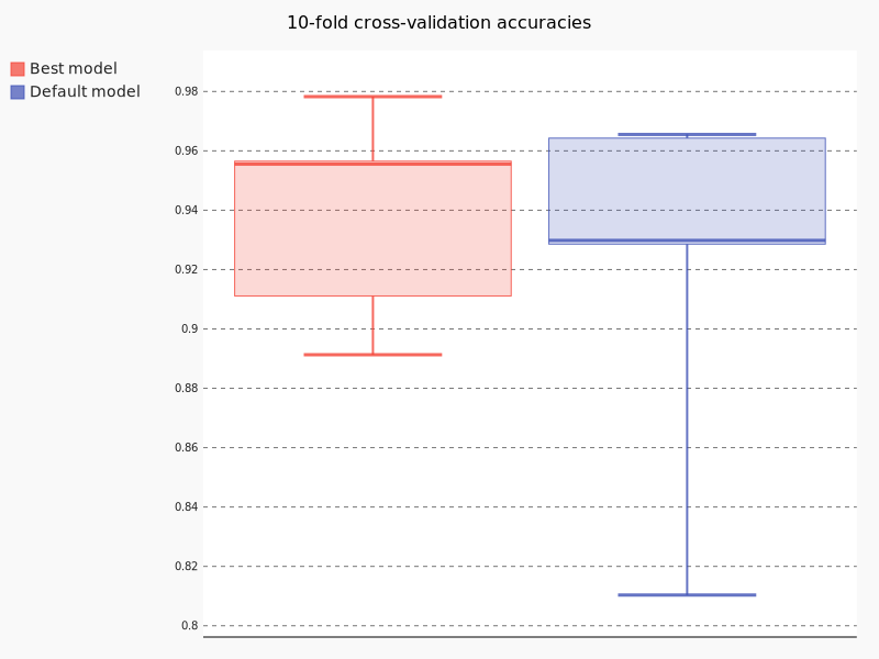
Aditionally, we can plot the results of each fold in form of the boxplot. Following is the snippet to plot such chart.
import pygal

box_plot = pygal.Box(width=800, height=600, range=(0.8, 0.99))
box_plot.zero = 0.9
box_plot.title = '10-fold cross-validation accuracies'
box_plot.add('Best model', model.ten_fold_scores['test_accuracy'])
box_plot.add('Default model', model.default_ten_fold_scores['test_accuracy'])

box_plot.render_to_png('chart.png')
Following Figure 2 is the output of previous code snippet. Observing the results of the default model and our model, we can see significant improvement in test accuracy using our model.
Final thoughts
In this post, you are guided through the process of utilizing the NiaPy micro-framework for purpose of finding the optimal parameters for K-nearest neighbors classifier. Additionally, the performance comparison between the classifier with default settings and classifier with optimal found parameters is performed and presented. The complete source code of the presented example can be found on the GitHub.
If you have any issues regarding the running or implementing the presented example, do not hesitate to comment or contact me.
References
Vrbančič, G., Brezočnik, L., Mlakar, U., Fister, D., & Fister Jr., I. (2018). NiaPy: Python microframework for building nature-inspired algorithms. Journal of Open Source Software, 3(23), 613. https://doi.org/10.21105/joss.00613 ↩︎ ↩︎
Cover, T., & Hart, P. (1967). Nearest neighbor pattern classification. IEEE transactions on information theory, 13(1), 21-27. ↩︎
Dua, D. and Karra Taniskidou, E. (2017). UCI Machine Learning Repository [http://archive.ics.uci.edu/ml]. Irvine, CA: University of California, School of Information and Computer Science. ↩︎
Fister Jr, I., Fister, D., & Yang, X. S. (2013). A hybrid bat algorithm. arXiv preprint https://arxiv.org/abs/1303.6310 ↩︎ ↩︎
Grega Vrbančič
Assistant Professor
Grega Vrbančič is an Assistant Professor at the University of Maribor, Faculty of Electrical Engineering and Computer Science.